"Comparing STOs and GTOs" Lab Procedure

Students

Procedure:

• For this lab, you will need access to a spreadsheet.

Part I:

Data Entry:

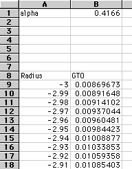
1. At the top of the spreadsheet, label the first cell "alpha." In the next cell define the constant.
2. Leaving a few rows blank, identify one cell "Radius." This is where we will give the equation various values of r.
3. Beneath Radius, you are going to create a list of values from -3 to +3. Divide the values into 0.01 increments. In order to do this, you are going to use a "Fill" comand. First, type a -3 in the first cell beneath the "Radius" label. Next, highlight the -3 and all the cells down to at least the 600th line. In the menu bar, look under Edit to find the "Fill" command. You want to choose the "Series" option. This will then prompt you for the increment by which you want your column to increase. The default is set to 1, but you will type 0.01. Click on OK. If your values do not reach +3, then repeat these steps until you reach this value.
4. Next to the Radius column, title the next cell "Gaussian" or "GTO."
5. Beneath this label you will need to enter you GTO function as given above. Remeber to identify alpha and the radius by their cell names and that pi=PI( ), e^x=EXP(x).

Hints:

• When referring to a cell, make sure you use, $, before the column or row if it remains constant.
• The first value should be 0.00869.

6. Use a "Fill" command, (this time use "Down" instead of "Series") in order to get values for all the radii.

Graphing:

1. Highlight the lists "Radius" and "GTO" including labels.
2. In the toolbar, click on the button with a wand and bar graph.
3. Select the area on the spreadsheet where you want the graph to appear.
4. Follow the steps to create a line graph.

Hints:

• In Excel, make sure you choose the XY scatter plot and the second type of line graph.

Part II:

1. Under alpha, type "xi." In the next cell, type the value.
2. Now, label the cell next to your GTO heading "Slater" or "STO." In the cell beneath the heading, enter the Slater equation. Fill down your column.

3. With the "Radius," "GTO," and "STO" columns highlighted, create a new graph to compare the GTO and STO calculations.
• Notice the major discrepency for small radii values. Also, notice how the approximations become similar for larger radii.

Part III:

To get all of the numerical constants required, we will have to use a basis set as a reference. These are stored in a large database, from which you can "order" a specific basis set.

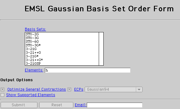
1. Go to the Gaussian Basis Set Order Format http://www.emsl.pnl.gov:2080/forms/basisform.html. Your browser should look like this: 
2. Order your constants:
• Select the STO-3G basis set. By selecting the STO-3G we are requesting to receive constants for 3 gaussians.
• Next type an h for hydrogen in the "Elements" blank.
• Don't put in an email!!
• Click Submit.
The result should be two columns of three numbers each. This is a basis set for hydrogen. The left list is alpha values, and the right list is coefficients which will be used to sum up the three gaussians.
3. Copy these constants so you can enter them into your spreadsheet.
4. At the top of your spreadsheet, next to the other constants, label each constant and define the value in the next cell.
5. Next to the STO column, put three new columns, labelled "g1," "g2," and "g3".
6. Under each new label, enter the gaussian equation using the values of alpha from the basis set and the radius as needed.
7. Fill down the column, and repeat the procedure for the other two columns.
8. Change the first number under Radius to be 0. When you do this, the whole list should change to go from 0 to 6 instead of -3 to 3. Also, the values in your gaussian lists should change, since we are computing them for different radii now. Check your values against those of your classmates to make sure you are all getting correct answers.

***Since we looked at the equations on both sides of the nucleus before, you should have observed that it is exactly the same on both sides. This is important! We are only interested in the positive side of the graph now, since we know that both sides will be exactly the same (and since negative and positive do not have any true physical meaning here!).***


9. Compare the answers from each new gaussian equation to those of the slater equation.

1. Create another column next to the three gaussians, labelled "LCAO".
2. Put the equation, referring to the appropriate constants, in the first cell.
3. Fill the column.

4. Create a graph of all three new gaussians and the LCAO.
5. To make this contrast clearer, we are going to examine several gaussian approximations and compare them to the STO.
6. Label three new columns for the two equations needed for a STO-2G model, and the STO-2G model itself.
7. Do the same for a STO-6G
8. Now go back to the order form for basis sets and find the basis sets, both alpha and d values, for STO-2G and STO-6G.
9. Put these values into your spreadsheet as before.
10. Set up each column with the neccessary equations.
11. In two new columns, use the LCAO equation for both of the 2G and 6G approximations.
12. Graph the 1 gaussian (the first one created), 2 G, 3 G , 6G, and STO all on a single graph. **DO NOT put all of the gaussians for each approximation on there, ONLY THE  SUMMATIONS.**