This page describes how to use the "GridSim Applet" (I don't know if that is the official name) and also some of the details of the internal workings of the applet and the underlying simulation. The overall goal of the applet is to let the user come to understand the trade-offs involved in running a simulation on a large computer or computer network. The user builds a network of computing resources, selects some parameters for the model to be run and then runs a simulation of the model. The simulation then reports back that the model took such and such time to run and cost xyz dollars, etc. By tuning the available knobs, the user is able to get a feel for the realities of both weather modelling and large-scale computing.
The applet in its current state may not quite reach this goal as it is necessary to tune not only the hardwired numbers in the applet, but also the way the applet does the simulation. The details of these "meta-knobs" will be discussed further down. The applet is by no means finished, but most of the core work is complete and, from my perspective, the rest of the work will involve tuning the applet to produce the right kind of output. That may not be an easy task...
When the applet begins, the user is presented with an empty "canvas", a "palette" of computing resources on the left, a blank information panel on the right and two buttons on the bottom. The first step to using the applet is building a network using the computing resources available. Currently, there are two types of computing resources: computers themselves and physical connections between them. The computers come in several flavors, which differ solely on the specs: speed of the processors, number of processors, amount of RAM, etc. If the user moves the mouse over one of the resources in the palette on the left, the information display on the right will show information specific to that resource.
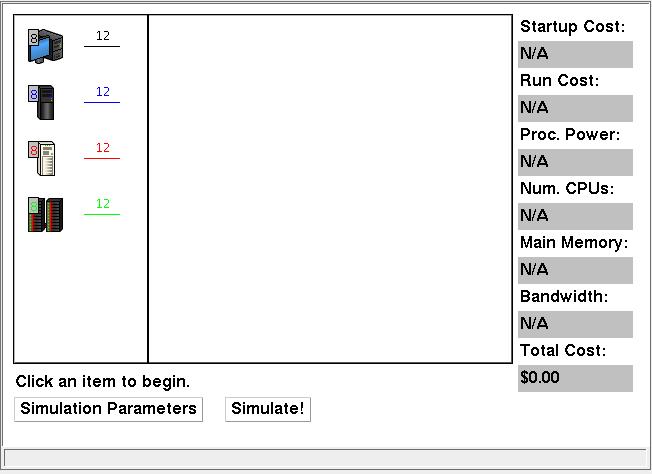
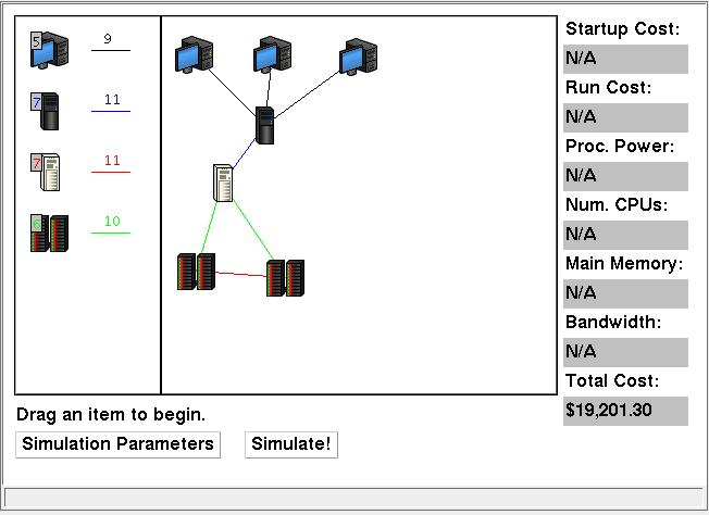
To actually build the network, the user must drag and drop resources from the palette onto the canvas in the middle. For computers, this is straightforward. In order to create a connection between two computers, the user must drag the connection resource from the palette to the starting computer and drop it there. Then, the user must click on the ending computer to complete the connection. At any time, adding a resource can be cancelled by clicking in the palette or dropping the item back in the palette. Items can be removed from the canvas by dragging them from the canvas back into the palette. If a computer is removed from the canvas, the applet automatically removes all connections going to that computer. As the network is built, the information panel on the right displays the cost of the network (at the bottom of the panel). This cost reflects the hardware cost of the network, that is, how much it would cost to buy all the equipment for the network and put it into place.
After the network is constructed, it is time to run the simulation. The simulation parameters must be set first in the simulation parameters dialog, which is brought up by clicking the "Simulation Parameters" button at the bottom of the applet. The dialog is as shown in the picture below:
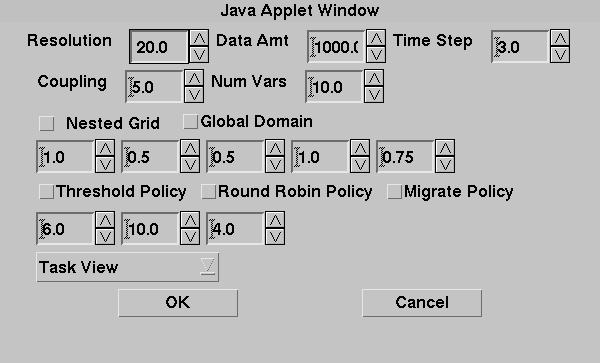
Firstly, the dialog will look prettier in the final version of the applet. The top five fields plus the two checkboxes labelled "nested grid" and "global domain" control aspects of the weather model to be simulated. Resolution basically determines how many parallel grid cells/points are modelled. Data Amt. is not used at the moment. Time step says how many iterations the model should go through. Coupling is a little bit ugly in the implementation, but basically says how much interaction there should be between parallel calculations. And number of variables says how many different variables should be taken into account during the modelling. If nested grid is checked, then the highest resolution is only for a chunk of the entire model domain near the middle, and areas outside of that have a lower resolution. Global domain just increase the resolution at the moment, but would later on imply that the model actually covers the whole Earth rather than just a small portion of it. See below for a discussion on the details of the simulation and how much work needs to be done to make it more realistic.
The remaining "knobs" control aspects of the task scheduler that is at the core of the simulation. Most, perhaps all, of these will be removed in the final version of the applet. The five unlabelled fields below "Nested Grid" are constants to a formula that helps the scheduler determine where to dispatch new tasks. They should not generally be messed with (but see below for the details in case you do want to mess with them). The next three checkboxes tell the scheduler to adopt a different policiy for dispatching tasks. Testing has shown that the default policy (all checkboxes cleared) is superior in most cases to using any of these policies. The fields below these checkboxes are parameters for the threshold and migrate policies respectively. The combo box at the very bottom determines how the simulation should display the usage patterns for each processor in the network (which will be explained next).
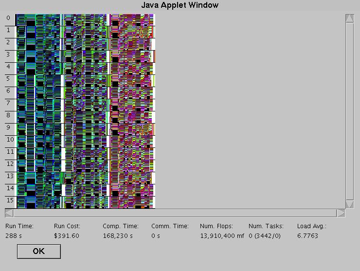
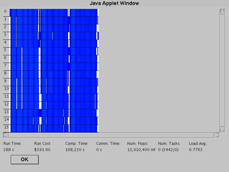
After setting the parameters for the simulation, it is necessary to actually run the simulation. The second button at the bottom of the applet is labelled "Simulate!" and this button starts the simulation using the parameters set in the simulation parameters dialog and the computing resources given in the network created by the user. A new dialog is displayed which not only provides the results of the simulation, but also shows the status of the simulation in real time. The big feature is a giant display showing the processor activity of all the processors in the network. The default display is "Task View", which means that the display shows which tasks are running on which processor. Each task has its own color. Due to the sheer number of tasks running in the model, the display is only useful for seeing how well the tasks are distributed across the processors (white indicates no tasks, meaning idle processors, meaning wastage) and also for eye-candy purposes. Below is a picture of the simulation dialog with "Task View" after a simulation has finished:
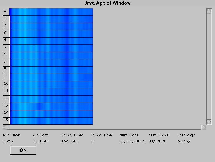
Another view is "Usage View", which shows instead how utilized the processors are, with white, again, indicating that the processor is idle. In many respects, this is much more useful than "Task View", although it isn't quite as exciting to look at, especially with low-intensity simulations.
And finally there is the "Load Average View", which also shows processor usage, but what it actually shows is the average utilization over the past 30 "ticks" of simulation. The result is a more smoothed version of the "Usage View". It may or may not be more useful than "Usage View", but it is prettier. There is also a "No Display" option, which does not have any graphical display of processor activity. At least on my machine, there is no large speedup in the amount of real time that the simulation takes, but your mileage may vary (my machine also is not that powerful).
The fields at the bottom of the dialog give some numbers related to the simulation as it is running and also after it is finished. From the left, there is "Run Time" which simply gives the number of seconds in simulated time that the model has taken to run. The Run Cost gives the total cost of running the model. Every tick that a processor is running the simulation costs X amount of money and every tick spent communicating between processors also costs some money. The "Comp. Time" and "Comm. Time" fields give the total amount of simulated time spent on running tasks and on communication respectively. The reason these numbers can be so large is that they are on a per processor basis. If processor 1 spends 323 ticks running tasks and processor 2 spends 485 ticks running tasks, then the Comp. Time field will show that 808 ticks were spent running tasks, even though the simulation may have finished in 500 ticks. The "Num Flops" field gives a rough estimate of how much computing work as actually done. Processors are assumed to run at 100% efficiency, so if a processor has a speed of 2 gigahertz, then a task running on that processor will execute 2 billion instructions per tick/second (in reality, it is obviously a lot less). Second to last is the "Num. Tasks" field which is really only useful during the simulation. It shows the number of tasks currently being executed at that moment in time and then, in parenthesis, the number of completed tasks and the number of tasks yet to run. Running tasks are not counted in either. And finally, the Load Average field displays the average number of tasks across all processors both during the simulation (when it is for the current tick) and after the simulation is complete (when it is averaged over the entire simulation).
That is pretty much all there is to using the applet. Playing with the network setup and the knobs for the simulation to get good results can obviously be a complex undertaking, however.
Besides the GUI, the applet has two main logical components: the computing network (implemented in the GCNetwork class) and the simulation engine (implemented in GCTaskScheduler, which relies on GCTaskGenerator). The GCNetwork class basically keeps track of what's present in the network. The information is stored in an adjacency matrix (see GCNetwork.java for the full details). GCTaskScheduler uses the data in GCNetwork to run the simulation.
The idea behind the simulation is that the weather model can be broken into atomic chunks representable by traditional tasks. The tasks run in parallel either on the same processor or on different ones. The details of uniprocessor multitasking are not simulated. Rather, the simulation simply allows for more than one task to be on a single processor and then adjusts the amount of time it takes for the task to complete based on the number of tasks running on the processor. Tasks have dependency relationships, which are only used when determining whether a task can start, not whether it can continue running. That is, a task may not be able to start until all its dependencies have completed, but once they have, the task is able to run and once it has started running, it does not stop and does not have to wait on any other tasks.
The number of tasks and the dependencies between them is determined by the parameters from the Simulation Parameters dialog. For example, the number of tasks created is related to the resolution (higher resolution means more tasks). GCTaskGenerator is the class in charge of generating a set of tasks to be run in the simulation. It is only run when the simulation parameters have changed.
A set of tasks basically looks like the following (with lines between tasks indicating dependency relationships):
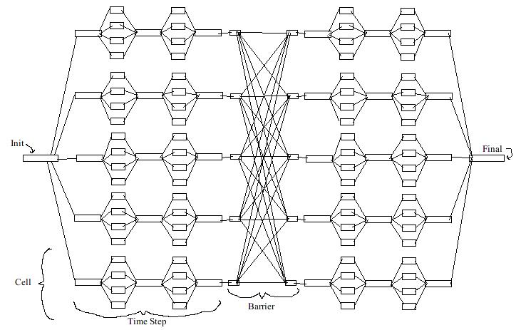
The first task is labelled "init". After it is complete, it spawns the cell init tasks. There is one for each cell. A cell is basically the smallest region represented by the model, but does not necessarily correspond to the model's gridpoint resolution. The cell init tasks then spawn the actual calculation tasks, one for each variable in the model. If the coupling value is greater than 1, then there are intermediate tasks that spawn off more calculation tasks. The idea behind these is that if the model coupling is high, then while modelling over the course of a time step, all of the parellel number cruching tasks should exchange answers more frequently. After all the tasks for a cell are complete, every cell plugs into a middle set of tasks called a barrier. The barrier is set up such that all the tasks of all the cells must complete before the model can go on to the next time step. Thus, a barrier defines the boundary between two time steps. When the model is finished, a finalization task is run and that's it.
Obviously, this model is extremely inaccurate compared to the real world. However, to a degree, it does the job of getting the right output. That is, if the model has a higher resolution, then it takes longer to run. Increasing the resolution also benefits from having more processors (since the cells run in parellel), whereas increasing the coupling or number of time steps will not often result in the model running significantly faster since time steps are run serially.
It has been mentioned that the parameters in the simulation parameters dialog control the simulation, but it hasn't yet been explained how. Below is a listing of how each of the parameters affects the simulation with respect to the number and arrangement of tasks:
The most obvious place for improvements is in the model. It is not so much that the model need be more complex or realistic, but that it must convey the realities and trade-offs inherent in large-scale computer modelling and weather modelling. It would perhaps be worthwhile to have a more complex picture of computing resources. As it stands now, the only focus is on processors, with some passing concern for how nodes are linked up. There are no routers, communication hubs and so forth. Neither are there data storage nodes and issues relating to that. A good question is whether it would even be worth it to consider these aspects. Would they bring too much complication to the applet without adding a whole lot? I don't have a good answer for that.
The interface could stand to look nicer, especially in the simulation parameters dialog. However, I think that the interface does a good job of providing necessary information in a reasonable fashion. I did try to put all the knobs to the simulation parameters dialog, rather than having them scattered all over the place. Earlier versions of the applet did have all of the interface on the main panel and this lead to a great deal of clutter among other issues. I do not think there is a whole lot of room for improvement in the applet interface, but others may disagree.