CASE STUDY: Smog Photochemistry Modeling

Source:

Model design by Dr. Kurt Peterson, Department of Environmental Engineering, Michigan Technological University. Used by permission. Narrative and case study design by Robert R. Gotwals, Jr.

WARNING! This case study requires a solid chemistry background AND the willingness to tackle a large, complex system that requires solid planning PRIOR to building the model with STELLA®. This model also REALLY requires you to pay attention to units and conversion of units.

Goal:

To learn about tropospheric photochemistry through modeling of urban ozone chemistry.

Background Reading:

Photochemical smog is an atmospheric condition that produces severe eye irritation and poor visibility, to name just two of the effects. Three ingredients -- energy from a light source (ultraviolet), hydrocarbons, and nitrogen oxides -- are needed for photochemical smog to be formed. Two of those components are produced through the burning of fossil fuels, most notably automobiles. Photochemical smog is also sometimes known as "oxidizing smog", in that it has a high concentration of oxidizing agents. Ozone is a common oxidizing agent found in photochemical smog. Another type of smog, reducing smog, has high concentrations of sulfur dioxide, which is a reducing agent. Its presence has historical significance in studies done in places like London, which used sulfur-containing coal as its main energy source.

A schematic is again useful in understanding the chemistry of smog production in the troposphere:

This graphic is relatively self-explanatory. It begins at the bottom with the production of NO and reactive hydrocarbons by fossil fuel burning (such as an automobile). On the left side, the NO reacts with tropospheric ozone or a hydrocarbon radical (RO_2•) to produce NO₂ (a radical is a molecule fragment that has an unpaired electron). This absorbs solar energy (represented by the letters "hv") to create NO (which propagates the system) and atomic oxygen. Atomic oxygen reacts to form tropospheric ozone, which feeds back into the NO_x system (the "x" here refers to the number of oxygens, and serves as a general notational term for the nitrogen oxides). Atomic oxygen can also react with hydroxyl radicals, OH•, and ozone to form the reactive hydrocarbon radicals utilized in the NO_x system. These radicals also react to form other components of smog, such as PAN (peroxyacetyl nitrate) and aldehydes (RC=OH, where R is some hydrocarbon chain).

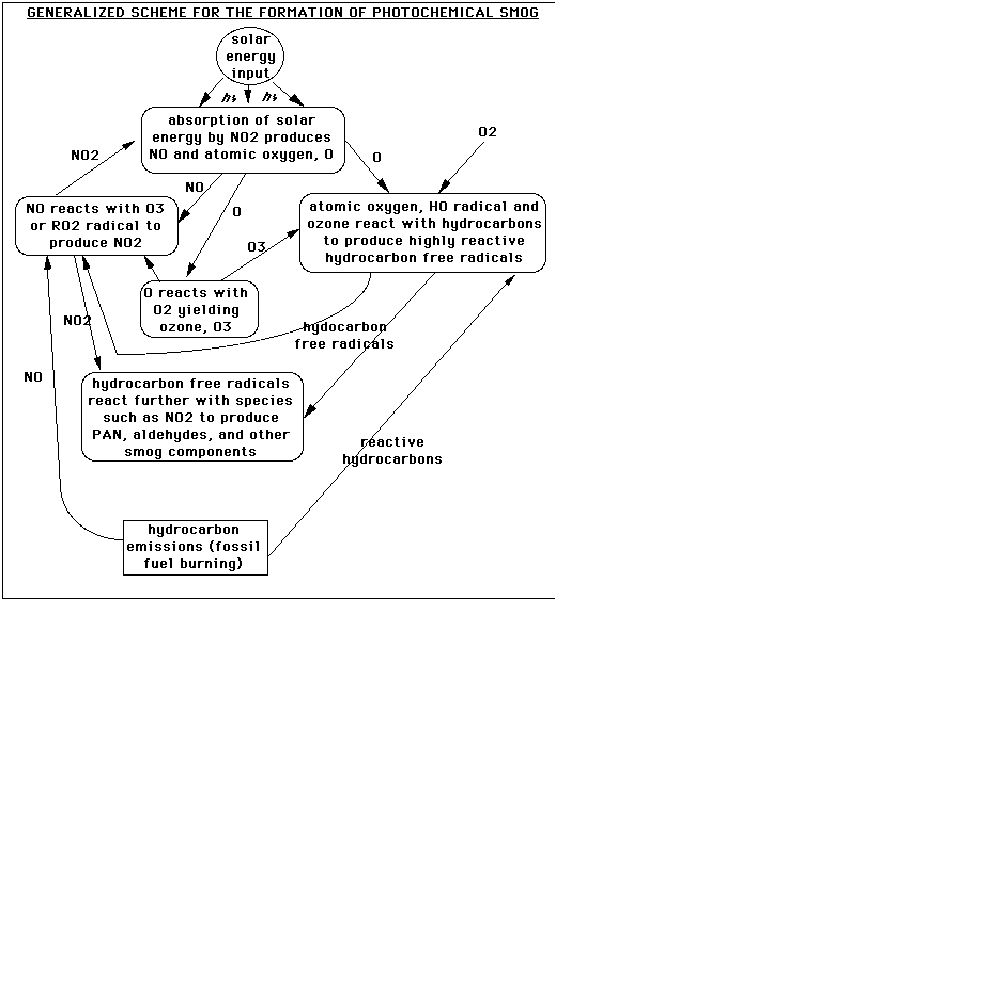
The graphic below shows the essential workings of the NOx system, with the interactions between NO and NO₂ on the left and the production/washout of HNO₃ on the right:

We can also look at the formation of photochemical smog from a kinetic perspective. This chart shows the nine key equations of smog production, and the rate constant that affects the speed (or rate) at which the reaction takes place:

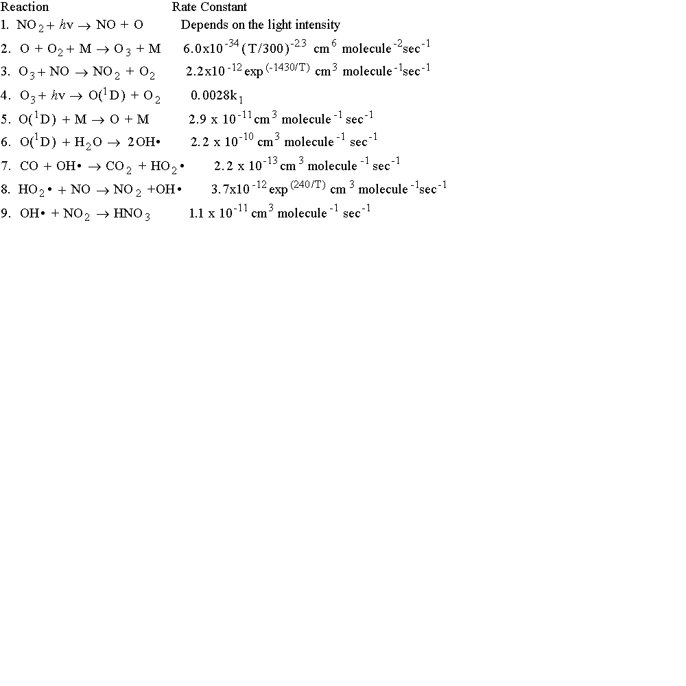
In this graphic, we see the involvement of the NO_x system and the production of ozone. Here is a narrative version of the graphic above:

Reaction 1: nitric oxide, NO₂, reacts with light energy, hv, to form nitrous oxide, NO and a singlet oxygen atom. The rate of this reaction depends on how much light energy there is -- a sunny day versus a cloudy day!
Reaction 2: singlet oxygen reacts with the oxygen molecule (what you breath) in the presence of a catalyst "M" to form ozone, O₃. The catalyst M remains unchanged (which is the definition of a catalyst!). The rate of this reaction depends on the temperature in the atmosphere.
Reaction 3: Ozone reacts with NO to produce more NO₂ and O₂. These products feed back into Reactions 1 and 2, thus ensuring a steady production of ozone! The rate of this reaction also depends on the temperature in the atmosphere.
Reaction 4: Ozone is degraded (broken down) by light energy, forming a charged form of singlet oxygen, O(1_D), and more molecular oxygen. Notice that this reaction proceeds at a much slower rate than the first reaction (about one-fourth of one percent as fast!)
Reaction 5: the charged oxygen reacts with a catalyst to return to its normal state of singlet oxygen (which is, by the way, poisonous to breathe!)
Reaction 6: some of the charged oxygen reacts with water in the atmosphere to form a hydroxyl radical, OH•. Radicals are fragments of molecules that have at least one unpaired electron, and are highly reactive. The hydroxyl radical, for example, is responsible for the majority of the chemical reactions that happen in the atmosphere during the day. Other radicals take control at night-time when there is no energy from the sun.
Reaction 7: carbon monoxide in the atmosphere, produced by fossil-fuel burning such as automobiles, reacts strongly with hydroxyl radicals to form carbon dioxide and HO₂• radicals.
Reaction 8: the HO₂• radicals formed in Reaction 7 react with the extra NO in the atmosphere to form more NO₂ and more OH• radicals. The rate of this reaction is dependent on the temperature in the atmosphere.
Reaction 9: the hydroxyl radicals react with NO₂ to form nitric acid, HNO₃, which will eventually be one of the culprits in the formation of acid rain, but that's (thankfully!) another model!

In summary: the development of photochemical smog is dependent upon solar radiation, source emissions of hydrocarbons and nitrogen oxides, and atmospheric stability (for enhanced concentrations). Early in the morning, commuter traffic releases NO and hydrocarbons. At the same time, NO₂ may decrease through because the sunlight can break it down to NO and O. The O is then free to react with O₂ to form O₃. Shortly thereafter, oxidized hydrocarbons react with NO to increase NO₂ by midmorning. This reaction causes NO to decrease and O₃ to build up, producing a midday peak in O₃ and minimum in NO. As the smog ripens, visibility may be reduced due to light scattering by aerosols. Primarily due to the dependence on commuter traffic between suburbs and cities, there are presently more than 40 urban areas in violation of the US ambient air quality standard for ozone.

We can look at the change in concentrations of NO, NO₂, and CO over time with this system of first-ordered differential equations. In the schematic below, we show the reactions by number from the graphic above. For example, R₁ represents the photochemical reaction in which light energy hits a molecule of NO₂ to form NO and singlet oxygen:

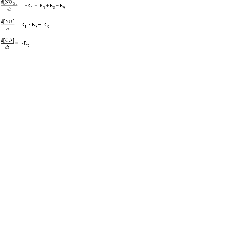
In the equations below, we substitute the kinetic components for each of the values of R:

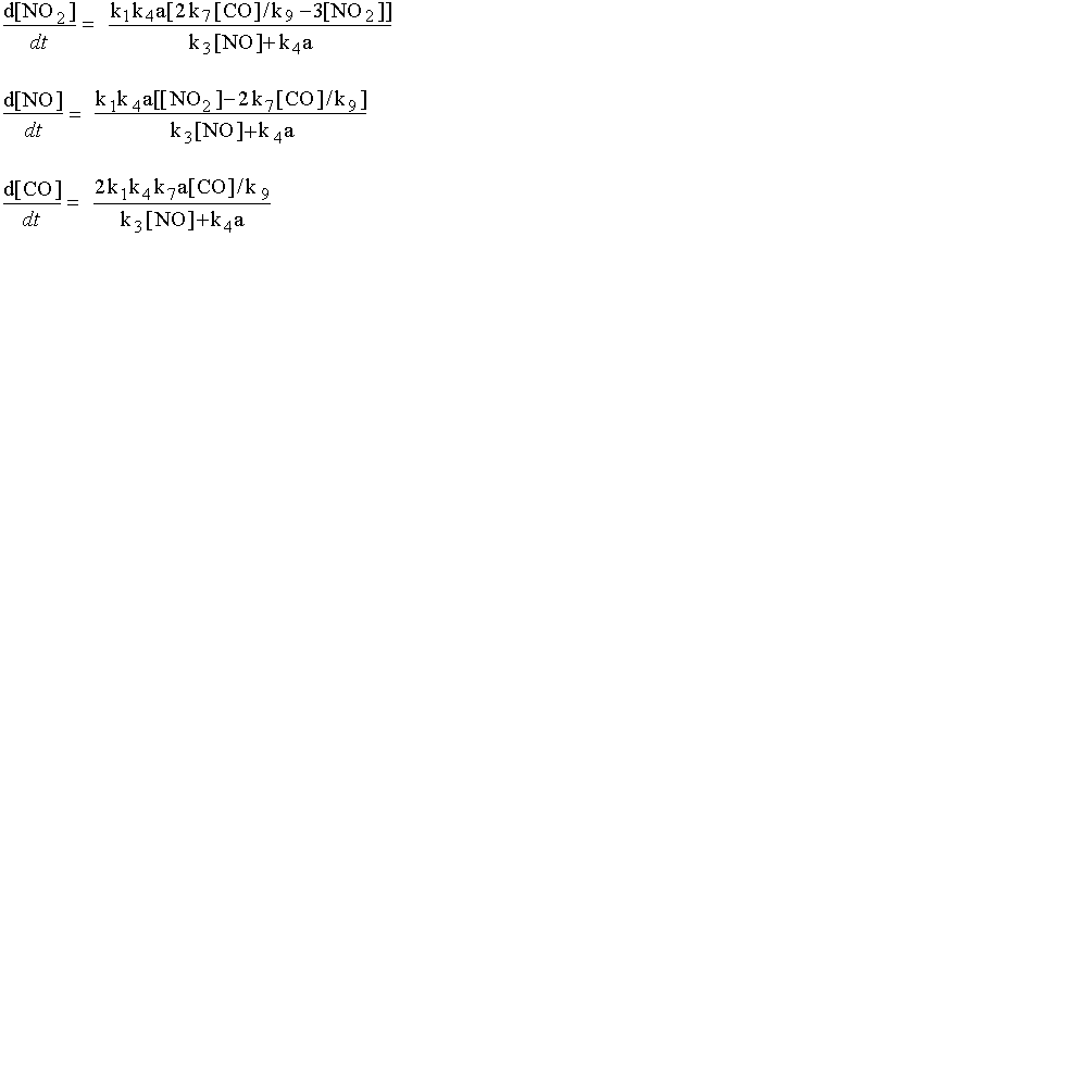
In these equations, the term "k" refers to the rate constants, and are numbered following the reaction numbers in the graphic above.

Building the Model:

Consider the photooxidation of CO in the presence of NO_x. Equations can be derived for [NO₂], [NO], and [CO], where the brackets [ ] mean "the concentration of". Integrate these equations numerically with STELLA for the following sets of conditions and plot [NO₂], [NO], [CO], and [O₃] in parts per billion (ppb) as a function of time from t=00 to t=180 minutes with a time step around 0.1 min for a stable solution. Use Runge-Kutta 4th Order solution. Assume T= 298 K (0 degrees Celsius is 273 degrees Kelvin, so 298 K is about 25 degrees Celsius, or about 80 degrees Fahrenheit, a nice warm day -- but you already knew how to do that conversion, didn't you!)

Initial Conditions (ppb)

TRIAL	1	2	3	4
[NO₂]_o	10	100	200	1000
[NO]_o	10	500	500	500
[CO]_o	50	10000	10000	10000

In each case assume that the photolysis rate constant for NO₂ (R1 above) is:

kNO₂ = 0.533 min^-1 (WARNING! Be careful with units here!)

In order for you to be able to build this model in a reasonable amount of time, I have done some of the algebraic rearrangements that need to be done to build this model in STELLA. You need to know that a "source" is an input, and a "sink" is an output.

Note that the reaction rates are in terms of molecules/cm³ not ppm, therefore your differential equations should work with molecules/cm³. Converters are used to translate molecule/cm³ to ppb (or ppm) which are more typical of air quality standards. Also many reaction rates are given as molecule/cm³-s, whereas the model is run in minutes.

Some other helpful info to use:

[H2O] = 0.3x10¹⁸ [molecule/cm³]
[M] = 0.2x10²⁰ [molecule/cm³]
k5=2.9x10^-11 cm³/molecule-sec
k6=2.2x10^-10 cm³/molecule-sec

Conversion factor:

1 molecule/cm³ = 4.08x10^-11 parts per billion (ppb)
All of the other k values needed -- k4, k7, k8, and k9 -- can be found on the table of reactions

**PAY CLOSE ATTENTION TO UNITS -- parts per billion, seconds, minutes, molecules/cm³, etc.

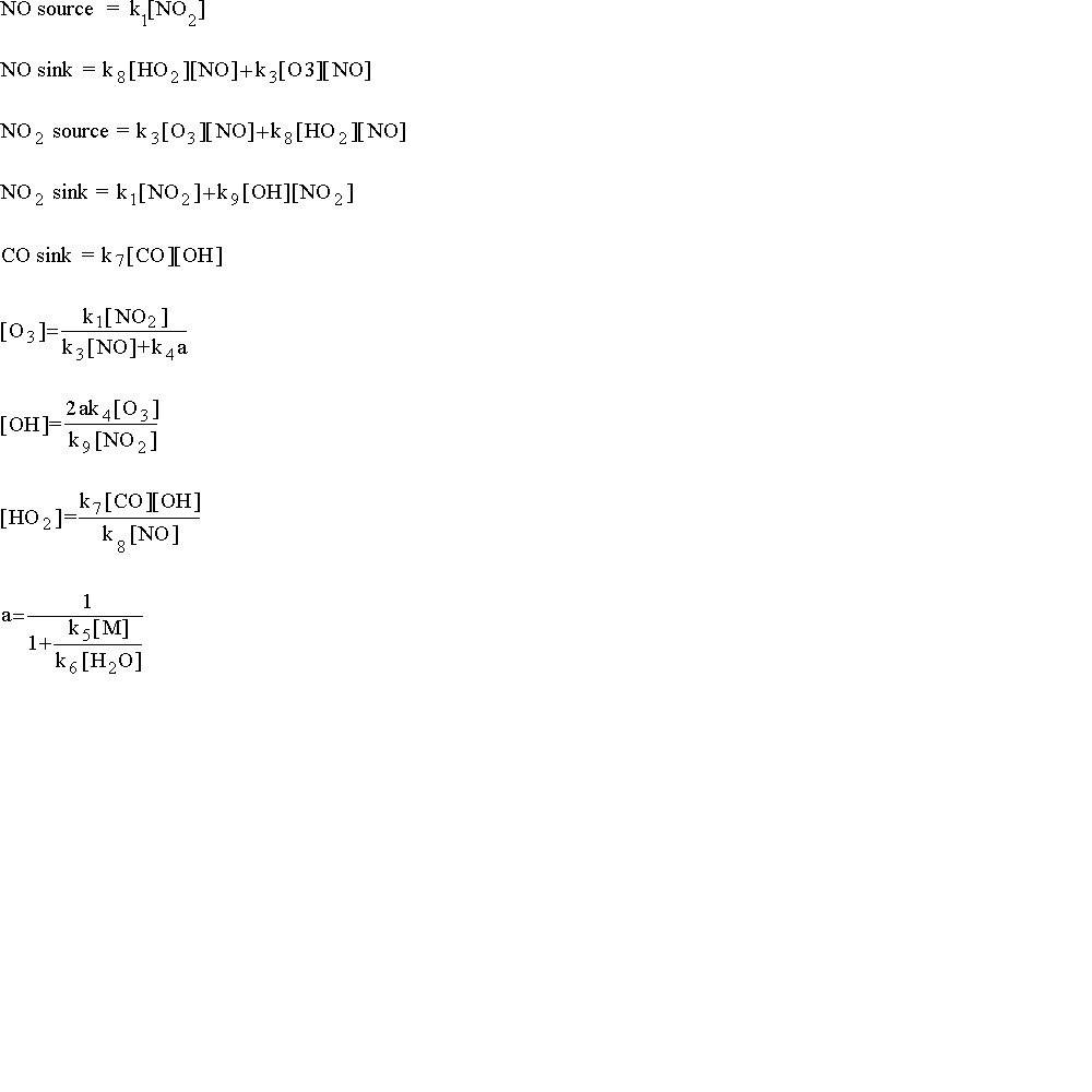
ALGORITHMS FOR SMOG PHOTOCHEMISTRY MODEL:

Once you have completed the model, experiment with various temperatures. You also might want to adjust the reaction rate of the first reaction, see what happens! You might also wish to run different starting values, such as are found in the Table of Inputs. If you have learned how, you might wish to consider doing multiple runs on one species.

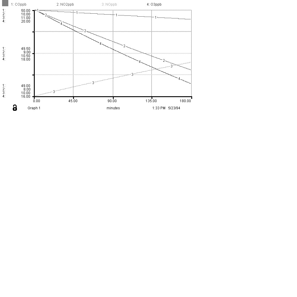
Below is a sample graph, in parts per billion, for the species of interest. Use this as a way to judge your model for accuracy and correctness.

SAMPLE RUN OF THE SMOG PHOTOCHEMISTRY MODEL (using Trial 1 starting points):

Developed by
Graphic of Shodor Logo