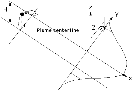
Gaussian Plume Model Application

One of the key assumptions of this model is that over short periods of time (such as a few hours), steady state conditions exist with regard to air pollutant emissions and meteorological changes. Air pollution is represented by an idealized plume coming from the top of a stack of some height and diameter. One of the primary calculations is the effective stack height. As the gases are heated in the plant (from the burning of coal or other materials), the hot plume will be thrust upward some distance above the top of the stack -- the effective stack height. We need to be able to calculate this vertical displacement, which depends on the stack gas exit velocity and temperature, and the temperature of the surrounding air.

Once the plume has reached its effective stack height, dispersion will begin in three dimensions. Dispersion in the downwind direction is a function of the mean wind speed blowing across the plume. Dispersion in the cross-wind direction and in the vertical direction will be governed by the Gaussian plume equations of lateral dispersion. Lateral dispersion depends on a value known as the atmospheric condition, which is a measure of the relative stability of the surrounding air. The model assumes that dispersion in these two dimensions will take the form of a normal Gaussian curve, with the maximum concentration in the center of the plume.

The graphic below shows a very simple schematic representation of the Gaussian plume model. At the top of the graphic is a smokestack which is emitting some amount of pollutant. The effective height of the emission (in meters) is the stack height plus the rise of the plume. The values of sigma y and sigma z represent the standard deviations of the horizontal and vertical distributions (respectively) of the pollutant. These distributions depend on a variety of meterological conditions, the most important being the stability category, which are dependent on wind speed, insolation, and the extent of the cloud cover. The model is called a Gaussian model since it has the mathematical shape of a Gaussian curve:

Initially, Gaussian plume models were used for pollutants such as carbon monoxide and other non-reactive species. The model has serious limitations when trying to account for pollutants that undergo chemical transformation in the atmosphere. Coupled with its dependence on steady state meteorological conditions and its short-term nature, this model has substantial limitations for use as a long-term airshed pollutant evaluator.